|
1
|
To define the condition, right-click a cross-tab element on which to display conditional formatting. From the menu, choose Format→Conditional Formatting.
|
|
2
|
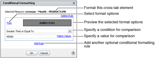
In Conditional Formatting, as shown in Figure 2-20, create a rule specifying the following information:
|
|
|
The condition that must be true to apply the format, such as revenue greater than or equal to 45000, as shown in Figure 2-20.
|
|
Figure 2-20
|
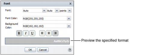
Figure 2-21 displays the choices of white text color (RGB(255,255,255)), gray background color (RGB(192,192,192)), and bold style on Font.
|
Figure 2-21
|
|
3
|
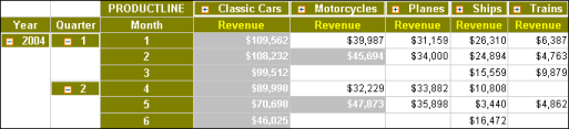
In Conditional Formatting, choose OK. In the cross tab in Figure 2-22, revenue values greater than or equal to $45,000 appear as bold, white text on a gray background.
|
|
4
|
To add another rule, right-click a cell and choose Format→Conditional Formatting. Then, on Conditional Formatting, choose Add Rule.
|
|
1
|
Right-click a cross-tab element. From the menu, choose Format→Conditional Formatting.
|
|
2
|
In Conditional Formatting, choose Delete Rule for each conditional formatting rule that you want to remove. Choose OK.
|