Using evolution

Video tutorial

An evolution analysis shows a progression of data over time. You can examine the behavior of certain measures in different periodic scenarios. For example, examine how the sales of some product families evolve over a period of months. The product family field is the categorical variable under study, while the different scenarios are determined by the different values in the month of purchase variable.

Define the following components to create an evolution analysis:

Categorical variable: Field that contains the categories whose behavior is to be analyzed, or in other words, the variable under study.

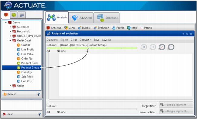
To indicate the variable you want to work with, drag the field from Data Tree to the control that is in the top part of the configuration form, as shown in Figure 4-18.

Figure 4-18

Control without variables

After dragging the variable to the control, it checks the number of discrete values and shows all of the divisions as well as the single values that it contains, as shown in Figure 4-19. Each green strip corresponds to a product type.

Figure 4-19

Control with variables

You can drag to this control only fields with a maximum of 100 discrete values. In the analysis, a sphere with a specific color selected at random represents each of these categories.

If you want to delete one or more of the categories from the analysis variable, click the box that represents the category. If you position the cursor over each of the green boxes, a tag appears, displaying the value of the option.

You can also select or deselect all of the boxes by using the buttons located just below the discrete values control (all, none).

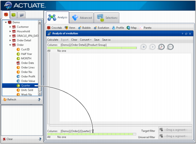
Measures: Evolution can display up to a maximum of three measures, two of which position the spheres on the axes of the x- and y- coordinates, while the third (optional) defines the relative measure of the sphere inside the group.

To define the measures of the axes, drag the numeric fields from Data Tree to the vertical bar (y-axis) or to the horizontal bar (x-axis).

When you drag a column to the x-axis, the latter changes color, indicating that it is ready to accept a column. After you drop the field, the control shows the applicable functions available in accordance with the type of column.

To use the third measure (sphere measure), drag the column you want to use to the icon that is located in the top-right part of the form.

If the cursor is positioned over the definition controls of the measures (axes, measure control), the current operation as well as the field involved in it are displayed.

Transition variable: It is necessary to define what data tree variable to use as a base for creating transitions. To indicate the field, you drag it to the discrete values control at the bottom of the form.

This control operates in the same way as the categorical variable control and enables you to indicate which elements to use in the analysis.

How to create an evolution

1	In Analytics—Analysis, choose Evolution.

2	From Data Tree, drag a column to use as the categorical variable, as shown in Figure 4-20.

Figure 4-20

Defining a categorical variable for an evolution analysis

3	From Data Tree, drag a column to use as the transition variable, as shown in Figure 4-21.

Figure 4-21

Defining a transition variable for an evolution analysis

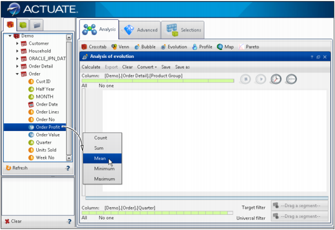
4	From Data Tree, drag columns onto the x-axis and y-axis. Choose appropriate functions for each axis. Figure 4-22 shows the y-axis being added as mean order profit with the x-axis in blue, to indicate that a column has already been applied.

Figure 4-22

Defining y-axis properties for an evolution analysis

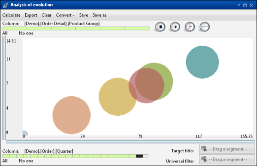
5	Choose Calculate. Choose Play to show the evolution over time. Figure 4-23 shows the evolution analysis.

Figure 4-23

Viewing an evolution analysis

6	To indicate a third measure, from Data Tree, drag a column to the far right icon.

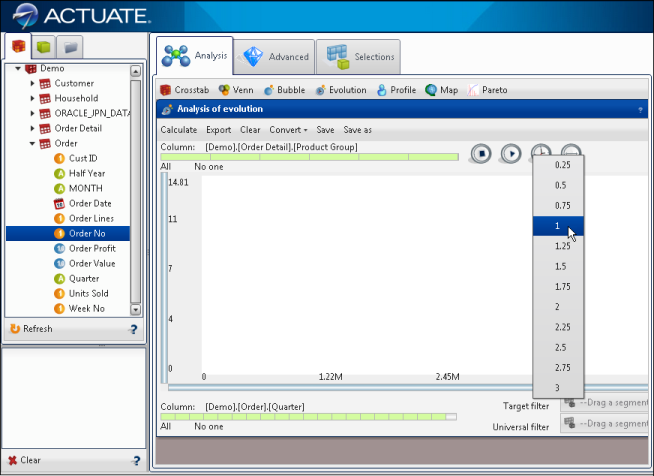
7	To modify the transition of time, select the clock icon and choose an interval, as shown in Figure 4-24. For example, an interval of 0.25 is faster than an interval of 3.

Figure 4-24

Editing the time dimension for an evolution analysis

More about viewing an evolution

When evolution is defined, BIRT Analytics internally creates a crosstab in which the categorical variable that you want to study is the row dimension (in the case of the example that accompanies this explanation, the product category) and the transition variable (the temporary variable) is the column dimension. The crosstab also includes the two or three defined measures (x, y, and measure).

The internal result of the crosstab is similar to Table 4-1.

Table 4-1

Internal result of crosstab

	Scenario 1				Scenario 2				Scenario 3
Category 1	x1	y1	measure1		x2	y2	measure2		x3	y3	measure3
Category 2	x1	y1	measure1		x2	y2	measure2		x3	y3	measure3

The graphic representation of the evolution analysis consists of data extracted from each of the scenarios, displayed as spheres. The animation extracts data from each scenario and displays each category as a sphere in a particular color, positioning it in a way that takes into account the maximum and minimum values of the measures for other categories.

During execution, you can hover the cursor over one of the spheres to display the name of the category and the values for each of its measures for the current transition. A transition is the category of the transition variable that is displayed by an evolution.

As the transitions occur, the active scenario of the transition variable appears.

It is possible to modify the time between transitions by choosing the time icon and selecting the speed.

The analysis definition form also allows you to set the filters for the calculation.

Recommendations

To make this analysis useful, the number of discrete values of the categorical variable must be as low as possible.

The analysis is deemed to exceed the maximum if it occupies more than one page.

To learn more about internal calculations, consult the crosstab help utility.

For example, consider the question, “How do the sales of a product family change over the months?” To answer this question, create an evolution indicating the group of products as a categorical variable and the month when the order is placed as a transitional variable. Possible measures are the orders count (x-axis) and the average profit (y-axis), which enable you to see quickly the group of products that sells most over time, and the group of products that produces the most profit. You can convert this type of analysis into a crosstab analysis.

Video tutorial

Creating a time evolution visualization

Copyright Actuate Corporation 2013

BIRT Analytics 4.2